Representing 2D Images#
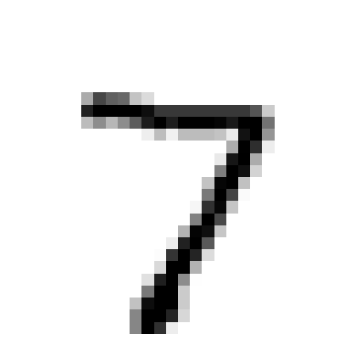
Now, suppose we have something like an image or a digit like the one below:
Show code cell source
import matplotlib.pyplot as plt
import numpy as np

digitPixels = np.reshape(np.array([0, 0, 0, 0, 0, 0, 0, 0, 0, 0, 0, 0, 0, 0, 0, 0, 0, 0, 0, 0, 0, 0, 0, 0, 0, 0, 0, 0, 0, 0, 0, 0, 0, 0, 0, 0, 0, 0, 0, 0, 0, 0, 0, 0, 0, 0, 0, 0, 0, 0, 0, 0, 0, 0, 0, 0, 0, 0, 0, 0, 0, 0, 0, 0, 0, 0, 0, 0, 0, 0, 0, 0, 0, 0, 0, 0, 0, 0, 0, 0, 0, 0, 0, 0, 0, 0, 0, 0, 0, 0, 0, 0, 0, 0, 0, 0, 0, 0, 0, 0, 0, 0, 0, 0, 0, 0, 0, 0, 0, 0, 0, 0, 0, 0, 0, 0, 0, 0, 0, 0, 0, 0, 0, 0, 0, 0, 0, 0, 0, 0, 0, 0, 0, 0, 0, 0, 0, 0, 0, 0, 0, 0, 0, 0, 0, 0, 0, 0, 0, 0, 0, 0, 0, 0, 0, 0, 0, 0, 0, 0, 0, 0, 0, 0, 0, 0, 0, 0, 0, 0, 0, 0, 0, 0, 0, 0, 0, 0, 0, 0, 0, 0, 0, 0, 0, 0, 0, 0, 0, 0, 0, 0, 0, 0, 0, 0, 0, 0, 0, 0, 0, 0, 84, 185, 159, 151, 60, 36, 0, 0, 0, 0, 0, 0, 0, 0, 0, 0, 0, 0, 0, 0, 0, 0, 0, 0, 0, 0, 0, 0, 222, 254, 254, 254, 254, 241, 198, 198, 198, 198, 198, 198, 198, 198, 170, 52, 0, 0, 0, 0, 0, 0, 0, 0, 0, 0, 0, 0, 67, 114, 72, 114, 163, 227, 254, 225, 254, 254, 254, 250, 229, 254, 254, 140, 0, 0, 0, 0, 0, 0, 0, 0, 0, 0, 0, 0, 0, 0, 0, 0, 0, 17, 66, 14, 67, 67, 67, 59, 21, 236, 254, 106, 0, 0, 0, 0, 0, 0, 0, 0, 0, 0, 0, 0, 0, 0, 0, 0, 0, 0, 0, 0, 0, 0, 0, 0, 83, 253, 209, 18, 0, 0, 0, 0, 0, 0, 0, 0, 0, 0, 0, 0, 0, 0, 0, 0, 0, 0, 0, 0, 0, 0, 0, 22, 233, 255, 83, 0, 0, 0, 0, 0, 0, 0, 0, 0, 0, 0, 0, 0, 0, 0, 0, 0, 0, 0, 0, 0, 0, 0, 0, 129, 254, 238, 44, 0, 0, 0, 0, 0, 0, 0, 0, 0, 0, 0, 0, 0, 0, 0, 0, 0, 0, 0, 0, 0, 0, 0, 59, 249, 254, 62, 0, 0, 0, 0, 0, 0, 0, 0, 0, 0, 0, 0, 0, 0, 0, 0, 0, 0, 0, 0, 0, 0, 0, 0, 133, 254, 187, 5, 0, 0, 0, 0, 0, 0, 0, 0, 0, 0, 0, 0, 0, 0, 0, 0, 0, 0, 0, 0, 0, 0, 0, 9, 205, 248, 58, 0, 0, 0, 0, 0, 0, 0, 0, 0, 0, 0, 0, 0, 0, 0, 0, 0, 0, 0, 0, 0, 0, 0, 0, 126, 254, 182, 0, 0, 0, 0, 0, 0, 0, 0, 0, 0, 0, 0, 0, 0, 0, 0, 0, 0, 0, 0, 0, 0, 0, 0, 75, 251, 240, 57, 0, 0, 0, 0, 0, 0, 0, 0, 0, 0, 0, 0, 0, 0, 0, 0, 0, 0, 0, 0, 0, 0, 0, 19, 221, 254, 166, 0, 0, 0, 0, 0, 0, 0, 0, 0, 0, 0, 0, 0, 0, 0, 0, 0, 0, 0, 0, 0, 0, 0, 3, 203, 254, 219, 35, 0, 0, 0, 0, 0, 0, 0, 0, 0, 0, 0, 0, 0, 0, 0, 0, 0, 0, 0, 0, 0, 0, 0, 38, 254, 254, 77, 0, 0, 0, 0, 0, 0, 0, 0, 0, 0, 0, 0, 0, 0, 0, 0, 0, 0, 0, 0, 0, 0, 0, 31, 224, 254, 115, 1, 0, 0, 0, 0, 0, 0, 0, 0, 0, 0, 0, 0, 0, 0, 0, 0, 0, 0, 0, 0, 0, 0, 0, 133, 254, 254, 52, 0, 0, 0, 0, 0, 0, 0, 0, 0, 0, 0, 0, 0, 0, 0, 0, 0, 0, 0, 0, 0, 0, 0, 61, 242, 254, 254, 52, 0, 0, 0, 0, 0, 0, 0, 0, 0, 0, 0, 0, 0, 0, 0, 0, 0, 0, 0, 0, 0, 0, 0, 121, 254, 254, 219, 40, 0, 0, 0, 0, 0, 0, 0, 0, 0, 0, 0, 0, 0, 0, 0, 0, 0, 0, 0, 0, 0, 0, 0, 121, 254, 207, 18, 0, 0, 0, 0, 0, 0, 0, 0, 0, 0, 0, 0, 0, 0, 0, 0, 0, 0, 0, 0, 0, 0, 0, 0, 0, 0, 0, 0, 0, 0, 0, 0, 0, 0, 0, 0, 0, 0, 0, 0, 0, 0]), (28, 28))


plt.figure()
plt.imshow(digitPixels, cmap='gray_r')
plt.axis('off')
plt.show()

We can represent this as a series of pixel values from 0 (blank) to 255 (filled in) and we can represent this as multiple Poisson variables with firing frequencies proportional to the value where \(Pr(spike) = T_{step}(\frac{d - d_{min}}{d_{max} - d_{min}} (r_{max} - r_{min}) + r_{min}\) where:
\(T_{step}\) is the size of time steps (e.g., \(0.001\) seconds)
\(d\) is the pixel value (\(0\) to \(255\))
\(d_{min}\) is the minimum pixel value (\(0\))
\(d_{max}\) is the maximum pixel value (\(255\))
\(r_{min}\) is the minimum firing rate (e.g., \(0\) Hz)
\(r_{max}\) is the maximum firing rate (e.g., \(1000\) Hz)
Our variable \(r_{min}\) can be thought of as the “noise”, since it controls how often the neurons in the background (the ones that are not part of the digit being represented) fire. Try modifying its value below:
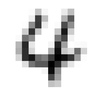
Visually, we can see that we can make out our numeric digit from the probabilitic firing patterns. However, if we increase \(r_{min}\), the background noise makes it more difficult to discern the represented digit. In code, we can create a function that generates the spikes for us, given an array values:
import random

def poisson_fire(values, min_value=0, max_value=255, min_rate=0, max_rate=10, dt=0.001):
    relativeValues    = [ (v - min_value) / (max_value - min_value) for v in values ] # Normalize values to [0, 1]
    relativeRates     = [ min_rate + v * (max_rate - min_rate) for v in relativeValues ] # Scale rates to [min_rate, max_rate]
    probabilityOfFire = [ r * dt for r in relativeRates ] # Probability of firing in each time step

    firings = [random.random() < p for p in probabilityOfFire] # Generate random firing events

    return firings
Show code cell source
im = [0, 0, 0, 0, 0, 0, 0, 0, 0, 0, 0, 0, 0, 0, 0, 0, 0, 0, 3, 57, 8, 0, 0, 20, 62, 0, 0, 0, 0, 0, 0, 0, 16, 185, 63, 0, 0, 75, 157, 0, 0, 0, 0, 0, 0, 2, 109, 188, 19, 0, 4, 169, 108, 0, 0, 0, 0, 0, 0, 47, 196, 56, 0, 0, 56, 220, 49, 0, 0, 0, 0, 0, 5, 134, 109, 1, 0, 0, 127, 176, 12, 0, 0, 0, 0, 0, 70, 205, 24, 0, 0, 11, 208, 91, 0, 4, 6, 0, 0, 0, 77, 199, 40, 0, 0, 79, 228, 54, 34, 138, 41, 0, 0, 0, 40, 199, 222, 140, 123, 186, 240, 225, 190, 94, 3, 0, 0, 0, 0, 31, 132, 159, 159, 243, 202, 86, 25, 2, 0, 0, 0, 0, 0, 0, 0, 0, 11, 231, 109, 0, 0, 0, 0, 0, 0, 0, 0, 0, 0, 0, 0, 173, 89, 0, 0, 0, 0, 0, 0, 0, 0, 0, 0, 0, 0, 59, 49, 0, 0, 0, 0, 0, 0, 0, 0, 0, 0, 0, 0, 0, 0, 0, 0, 0, 0, 0]

num_firings = [0] * len(im)

for i in range(1000):
    firings = poisson_fire(im, max_rate=100)
    for j in range(len(im)):
        if firings[j]:
            num_firings[j] += 1
Show code cell source
import matplotlib.pyplot as plt
import numpy as np

plt.figure()
# plot im as a 14x14 matrix
plt.imshow(np.reshape(im, (14, 14)), cmap='gray_r')
plt.axis('off')
plt.show()

Summary#
We often model data sources as Poisson processes
These models can represent values as probabilistic frequencies
We can represent 2D images as a neuron group where each neuron represents a different pixel in the image
