Adaptive LIF Neurons#
Thusfar, in modeling leaky integrate-and-fire (LIF) neurons, the only state variable that we have been modifying has been its current voltage/potential. However, in some applications it can also be useful to allow the threshold voltage (\(v_{th}\)) to vary. Specifically, when there is a spike, we can slightly increase \(v_{th}\) so that it is slightly more difficult to spike next time (i.e., it adapts to the level of input). We will call our new neuron model “Adaptive LIF” (ALIF).
The ALIF can be useful in a variety of scenarios, including cases where we want neurons to “fine tune” their behave to adapt to input that might otherwise be too “intense” (and thus result in too high of a firing rate if neurons don’t adapt) and cases where we want to be sure that one neuron in a group doesn’t get “greedy” for inputs with which it is closely aligned.
To implement ALIF neurons, we will create an additional state variable \(w\) to represent how much the threshold voltage (\(v_{th}\)) has increased (meaning that we will spike only when \(v \geq v_{th} + w\)). \(w\) will start as \(0\) and increase every time our neuron fires. We also create a variable \(b\) to represent the strength of adaption. When our ALIF spikes, we will increment \(w\) by \(b\). We will also introduce a time constant \(\tau_w\) to specify how quickly \(w\) decays back to \(0\).
So now, rather than a static threshold \(v_{th}\), we have a dynamic threshold, which we will call \(\vartheta_{th}(t)\):
\(\vartheta_{th}(t) = v_{th} + w(t)\)
and our threshold changes over time by:
\(\vartheta_{th}'(t) = -\frac{1}{\tau_w}w(t)\)
if there is a spike at time \(t\) then \(w(t)\) increases by \(b\).
To implement ALIF neurons, let’s start by recalling the code that we had for LIF neurons:
class LIF:
    def __init__(self, n=1, dim=1, tau_rc=0.02, tau_ref=0.002, v_th=1,
                 max_rates=[200, 400], intercept_range=[-1, 1], t_step=0.001, v_init = 0):
        self.n = n
        # Set neuron parameters
        self.dim = dim  # Dimensionality of the input
        self.tau_rc = tau_rc  # Membrane time constant
        self.tau_ref = tau_ref  # Refractory period
        self.v_th = np.ones(n) * v_th  # Threshold voltage for spiking
        self.t_step = t_step  # Time step for simulation

        # Initialize state variables
        self.voltage = np.ones(n) * v_init  # Initial voltage of neurons
        self.refractory_time = np.zeros(n)  # Time remaining in refractory period
        self.output = np.zeros(n)  # Output spikes

        # Generate random max rates and intercepts within the given range
        max_rates_tensor = np.random.uniform(max_rates[0], max_rates[1], n)
        intercepts_tensor = np.random.uniform(intercept_range[0], intercept_range[1], n)

        # Calculate gain and bias for each neuron
        self.gain = self.v_th * (1 - 1 / (1 - np.exp((self.tau_ref - 1/max_rates_tensor) / self.tau_rc))) / (intercepts_tensor - 1)
        self.bias = np.expand_dims(self.v_th - self.gain * intercepts_tensor, axis=1)

        # Initialize random encoders
        self.encoders = np.random.randn(n, self.dim)
        self.encoders /= np.linalg.norm(self.encoders, axis=1)[:, np.newaxis]

    def reset(self):
        # Reset the state variables to initial conditions
        self.voltage = np.zeros(self.n)
        self.refractory_time = np.zeros(self.n)
        self.output = np.zeros(self.n)

    def step(self, inputs):
        dt = self.t_step  # Time step

        # Update refractory time
        self.refractory_time -= dt
        delta_t = np.clip(dt - self.refractory_time, 0, dt) # ensure between 0 and dt

        # Calculate input current
        I = np.sum(self.bias + inputs * self.encoders * self.gain[:, np.newaxis], axis=0) / self.n

        # Update membrane potential
        self.voltage = I + (self.voltage - I) * np.exp(-delta_t / self.tau_rc)

        # Determine which neurons spike
        spike_mask = self.voltage > self.v_th
        self.output[:] = spike_mask / dt  # Record spikes in output

        # Calculate the time of the spike
        t_spike = self.tau_rc * np.log((self.voltage[spike_mask] - I[spike_mask]) / (self.v_th[spike_mask] - I[spike_mask])) + dt

        # Reset voltage of spiking neurons
        self.voltage[spike_mask] = 0

        # Set refractory time for spiking neurons
        self.refractory_time[spike_mask] = self.tau_ref + t_spike

        return self.output  # Return the output spikes
On top of this code, we will add:
inhto represent \(w\), a variable that tracks how much the threshold voltage (v_th) has increased (meaning thatvwill need to exceedthis.v_th + this.inh)tau_inhto represent \(\tau_w\), a time constant that tracks howinhshould evolve over timeinc_inhto represent \(b\), which specifies how much to increaseinhevery time the neuron spikes
We can update our constructor to include defaults for tau_inh and inc_inh (0.05 and 1 respectively):
constructor(... tau_inh = 0.05, inc_inh = 1) ...
and initializing our instance variables (with this.inh initialized to 0):
self.inh = 0;
self.tau_inh = tau_inh;
self.inc_inh = inc_inh;
Now, we want to update our firing condition (if(this.v > this.v_th)) to add this.inh:
if self.v >= self.v_th + self.inh: #...
and we want to update self.inh every timestep:
self.inh = self.inh * (1 - t_step/self.tau_inh);
and if we fire:
    if self.v >= self.v_th + self.inh:
        self.inh += self.inc_inh
        #...
Below is the full code with these changes incorporated:
Show code cell source
import numpy as np

class ALIF:
    def __init__(self, n=1, dim=1, tau_rc=0.02, tau_ref=0.002, v_th=1,
                 max_rates=[200, 400], intercept_range=[-1, 1], t_step=0.001, v_init = 0,
                 tau_inh=0.05, inc_inh=1.0 # <--- ADDED
                 ):
        self.n = n
        # Set neuron parameters
        self.dim = dim  # Dimensionality of the input
        self.tau_rc = tau_rc  # Membrane time constant
        self.tau_ref = tau_ref  # Refractory period
        self.v_th = np.ones(n) * v_th  # Threshold voltage for spiking
        self.t_step = t_step  # Time step for simulation

        self.inh = np.zeros(n)  # <--- ADDED
        self.tau_inh = tau_inh  # <--- ADDED
        self.inc_inh = inc_inh  # <--- ADDED

        # Initialize state variables
        self.voltage = np.ones(n) * v_init  # Initial voltage of neurons
        self.refractory_time = np.zeros(n)  # Time remaining in refractory period
        self.output = np.zeros(n)  # Output spikes

        # Generate random max rates and intercepts within the given range
        max_rates_tensor = np.random.uniform(max_rates[0], max_rates[1], n)
        intercepts_tensor = np.random.uniform(intercept_range[0], intercept_range[1], n)

        # Calculate gain and bias for each neuron
        self.gain = self.v_th * (1 - 1 / (1 - np.exp((self.tau_ref - 1/max_rates_tensor) / self.tau_rc))) / (intercepts_tensor - 1)
        self.bias = np.expand_dims(self.v_th - self.gain * intercepts_tensor, axis=1)

        # Initialize random encoders
        self.encoders = np.random.randn(n, self.dim)
        self.encoders /= np.linalg.norm(self.encoders, axis=1)[:, np.newaxis]

    def reset(self):
        # Reset the state variables to initial conditions
        self.voltage = np.zeros(self.n)
        self.refractory_time = np.zeros(self.n)
        self.output = np.zeros(self.n)
        self.inh = np.zeros(self.n)  # <--- ADDED

    def step(self, inputs):
        dt = self.t_step  # Time step

        # Update refractory time
        self.refractory_time -= dt
        delta_t = np.clip(dt - self.refractory_time, 0, dt) # ensure between 0 and dt

        # Calculate input current
        I = np.sum(self.bias + inputs * self.encoders * self.gain[:, np.newaxis], axis=1)

        # Update membrane potential
        self.voltage = I + (self.voltage - I) * np.exp(-delta_t / self.tau_rc)

        # Determine which neurons spike
        spike_mask = self.voltage > self.v_th + self.inh  # <--- ADDED + self.inh
        self.output[:] = spike_mask / dt  # Record spikes in output

        # Calculate the time of the spike
        t_spike = self.tau_rc * np.log((self.voltage[spike_mask] - I[spike_mask]) / (self.v_th[spike_mask] - I[spike_mask])) + dt

        # Reset voltage of spiking neurons
        self.voltage[spike_mask] = 0

        # Set refractory time for spiking neurons
        self.refractory_time[spike_mask] = self.tau_ref + t_spike

        self.inh = self.inh * np.exp(-dt / self.tau_inh) + self.inc_inh * (self.output > 0)  # <--- ADDED

        return self.output  # Return the output spikes
Let’s see what this looks like with tau_inh = 0.3 and inc_inh = 0.2 over a short time period (0.5 seconds). Note that we reduced the neuron’s refractory period so that the effect is more visible:
Show code cell source
import matplotlib.pyplot as plt

T = 5
t_step = 0.001
neurons = ALIF(n=1, t_step=t_step, tau_inh=0.3, inc_inh=0.2)
neurons.bias = np.array([0]) ; neurons.gain = np.array([1]) ; neurons.encoders = np.array([[1]]) # Remove the random gain, bias, and encoders

times = np.arange(0, T, t_step)
inp = 1.3

outputs = []
for t in times:
    neurons.step(inp)
    outputs.append((neurons.voltage[0], neurons.v_th[0] + neurons.inh[0], neurons.output[0]))

short_n = round(0.5 / t_step)
plt.figure()
plt.plot(times[:short_n], [o[0] for o in outputs[:short_n]], color='red', label='Voltage')
plt.plot(times[:short_n], [o[1] for o in outputs[:short_n]], color='blue', label='Threshold', linestyle='--')
plt.plot(times[:short_n], [o[2] * t_step for o in outputs[:short_n]], linewidth=4, color='black', label='Output')
plt.legend()
plt.show()
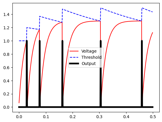
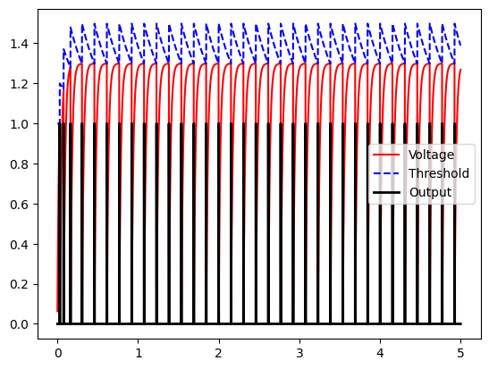
Note that at first, the neuron spikes quickly but then spikes become more spaced out over time. The firing speed does become more regular over the long term, as our threshold and voltage “balance” out. Let’s look over a period of 5 seconds:
Show code cell source
plt.figure()
plt.plot(times, [o[0] for o in outputs], color='red', label='Voltage')
plt.plot(times, [o[1] for o in outputs], color='blue', label='Threshold', linestyle='--')
plt.plot(times, [o[2] * t_step for o in outputs], linewidth=2, color='black', label='Output')
plt.legend()
plt.show()
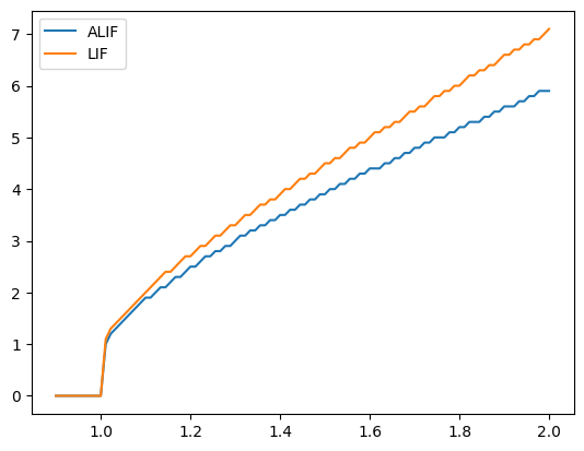
Finally, we claimed that part of the motivation for using ALIFs is that their firing rate can be less sensitive to input variability…so let’s test this. Again, to make the difference more visible, we are going to tune a parameter of our ALIF neurons…we are going to increase tau_inh to 0.7 so that the additional inhibition stays for “longer” after it is increased.
Show code cell source
def plotFiringRates(tau_inh, inc_inh):
    t_step = 0.001
    def getFiringRate(inp, neuron, runtime=10):
        times = np.arange(0, runtime, t_step)
        num_spikes = 0
        for t in times:
            neuron.step(inp)
            if neuron.output[0] > 0:
                num_spikes += 1
        return num_spikes / runtime

    alifs = ALIF(n=1, tau_ref=0.002, tau_rc=0.2, t_step=t_step, tau_inh=tau_inh, inc_inh=inc_inh)
    lifs  =  LIF(n=1, tau_ref=0.002, tau_rc=0.2, t_step=t_step)

    alifs.bias = lifs.bias = np.array([0]) ; alifs.gain = lifs.gain = np.array([1]) ; alifs.encoders = lifs.encoders = np.array([[1]]) # Remove the random gain, bias, and encoders

    rates = []

    for inp in np.linspace(0.9, 2, 100):
        alifFiringRate = getFiringRate(inp, alifs)
        lifFiringRate  = getFiringRate(inp, lifs)

        alifs.reset() ; lifs.reset()
        rates.append((inp, alifFiringRate, lifFiringRate))

    plt.figure()
    plt.plot([r[0] for r in rates], [r[1] for r in rates], label='ALIF')
    plt.plot([r[0] for r in rates], [r[2] for r in rates], label='LIF')
    plt.legend()
    plt.show()
plotFiringRates(tau_inh=0.7, inc_inh=1.0)
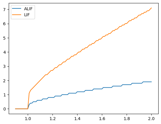
Note here how the ALIF (blue line) is less sensitive to changes in input than the normal LIF. If we decrease tau_inh, our ALIF behaves more and more like the LIF model (since the inhibition disappears more quickly).
plotFiringRates(tau_inh=0.3, inc_inh=1.0)
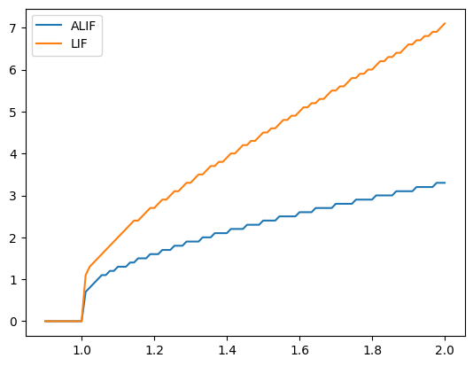
Similarly, if we decrease inc_inh, our ALIF behaves more and more like the LIF model (since the inhibition changes less).
plotFiringRates(tau_inh=0.3, inc_inh=0.1)
Summary#
Adaptive LIF neurons introduce a variable firing threshold \(\vartheta_{th}(t) = v_{th} + w(t)\)
\(v_{th}\) is the “original” firing threshold
\(w_{t}\) is an additional threshold that changes over time: \(w'(t) = -\frac{1}{\tau_w}w(t)\)
\(\tau_w\) is a time constant that controls how quickly \(w(t)\) decays
if there is a spike at time \(t\) then \(w(t)\) increases by some constant \(b\).
Adaptive LIFs can help us make our LIFs’ firing rate less sensitive to input variability