Research Replication: Unsupervised Learning of Digit Recognition Using STDP (Part 2)#
In our last tutorial, we designed an SNN to classify digits. We used the MNIST dataset for training. However, we used a scaled down model for illustration. In this notebook, we’re going to scale up the model a bit (though not to the full scale in the paper). We are going to use 400 excitatory and inhibitory neurons, 28x28 digits, and pre-trained weights (from here).
First, let’s take a look at what our pre-trained STDP weights look like. Below, in a grid, we can see what the input weights for all 400 neurons look like.
Show code cell content
from myst_nb import glue
import numpy as np

np.random.seed(0)

NUM_NEURONS = 400
NUM_NEURON_COLS = 20
NUM_NEURON_ROWS = 20

DIGIT_WIDTH =28
DIGIT_HEIGHT=28
DIGIT_SIZE=DIGIT_WIDTH*DIGIT_HEIGHT

glue("NUM_NEURONS", NUM_NEURONS, display=False)
glue("NUM_NEURON_COLS", NUM_NEURON_COLS, display=False)
glue("NUM_NEURON_ROWS", NUM_NEURON_ROWS, display=False)
glue("DIGIT_SIZE", DIGIT_SIZE, display=False)
glue("DIGIT_WIDTH", DIGIT_WIDTH, display=False)
glue("DIGIT_HEIGHT", DIGIT_HEIGHT, display=False)

def poisson_fire(values, min_value=0, max_value=255, min_rate=0, max_rate=10, dt=0.001):
    relativeValues = (values - min_value) / (max_value - min_value)
    relativeRates = min_rate + relativeValues * (max_rate - min_rate)
    probsOfFire = relativeRates * dt

    firings = np.random.rand(*values.shape) < probsOfFire
    return firings / dt

class SynapseCollection:
    def __init__(self, n=1, tau_s=0.05, t_step=0.001):
        self.n = n
        self.a = np.exp(-t_step / tau_s)  # Decay factor for synaptic current
        self.b = 1 - self.a  # Scale factor for input current

        self.voltage = np.zeros(n)  # Initial voltage of neurons

    def step(self, inputs):
        self.voltage = self.a * self.voltage + self.b * inputs

        return self.voltage

class STDPWeights:
    def __init__(self, numPre, numPost, tau_plus = 0.03, tau_minus = 0.03, a_plus = 0.1, a_minus = 0.11, g_min=0, g_max=1):
        self.numPre = numPre
        self.numPost = numPost
        self.tau_plus = tau_plus
        self.tau_minus = tau_minus
        self.a_plus = a_plus
        self.a_minus = a_minus
        self.x = np.zeros(numPre)
        self.y = np.zeros(numPost)

        self.g_min = g_min
        self.g_max = g_max
        self.w = np.random.uniform(g_min, g_max, (numPre, numPost)) / numPost # Initialize weights


    def step(self, t_step):
        self.x = self.x * np.exp(-t_step/self.tau_plus)
        self.y = self.y * np.exp(-t_step/self.tau_minus)

    def updateWeights(self, preOutputs, postOutputs):
        self.x += (preOutputs  > 0) * self.a_plus
        self.y -= (postOutputs > 0) * self.a_minus

        alpha_g = self.g_max - self.g_min # Scaling factor for weight updates

        preSpikeIndices = np.where(preOutputs > 0)[0]   # Indices of pre-synaptic   spiking neurons
        postSpikeIndices = np.where(postOutputs > 0)[0]

        for ps_idx in preSpikeIndices:
            self.w[ps_idx] += alpha_g * self.y
            self.w[ps_idx] = np.clip(self.w[ps_idx], self.g_min, self.g_max)

        for ps_idx in postSpikeIndices:
            self.w[:, ps_idx] += alpha_g * self.x
            self.w[:, ps_idx] = np.clip(self.w[:, ps_idx], self.g_min, self.g_max)

class LIF:
    def __init__(self, n=1, dim=1, tau_rc=0.02, tau_ref=0.002, v_th=1,
                 max_rates=[200, 400], intercept_range=[-1, 1], t_step=0.001, v_init = 0):
        self.n = n
        # Set neuron parameters
        self.dim = dim  # Dimensionality of the input
        self.tau_rc = tau_rc  # Membrane time constant
        self.tau_ref = tau_ref  # Refractory period
        self.v_th = np.ones(n) * v_th  # Threshold voltage for spiking
        self.t_step = t_step  # Time step for simulation

        # Initialize state variables
        # self.voltage = np.ones(n) * v_init  # Initial voltage of neurons
        self.voltage = np.random.uniform(0, 1, n)  # Initial voltage of neurons
        self.refractory_time = np.zeros(n)  # Time remaining in refractory period
        self.output = np.zeros(n)  # Output spikes

        # Generate random max rates and intercepts within the given range
        max_rates_tensor = np.random.uniform(max_rates[0], max_rates[1], n)
        intercepts_tensor = np.random.uniform(intercept_range[0], intercept_range[1], n)

        # Calculate gain and bias for each neuron
        # self.gain = self.v_th * (1 - 1 / (1 - np.exp((self.tau_ref - 1/max_rates_tensor) / self.tau_rc))) / (intercepts_tensor - 1)
        # self.bias = np.expand_dims(self.v_th - self.gain * intercepts_tensor, axis=1)
        self.gain = np.ones(n)
        self.bias = np.zeros(n)

        # Initialize random encoders
        # self.encoders = np.random.randn(n, self.dim)
        # self.encoders /= np.linalg.norm(self.encoders, axis=1)[:, np.newaxis]
        self.encoders = np.ones((n, self.dim))

    def reset(self):
        # Reset the state variables to initial conditions
        self.voltage = np.zeros(self.n)
        self.refractory_time = np.zeros(self.n)
        self.output = np.zeros(self.n)

    def step(self, inputs):
        dt = self.t_step  # Time step

        # Update refractory time
        self.refractory_time -= dt
        delta_t = np.clip(dt - self.refractory_time, 0, dt) # ensure between 0 and dt

        # Calculate input current
        I = np.sum(self.bias + inputs * self.encoders * self.gain[:, np.newaxis], axis=0) / self.n

        # Update membrane potential
        self.voltage = I + (self.voltage - I) * np.exp(-delta_t / self.tau_rc)

        # Determine which neurons spike
        spike_mask = self.voltage > self.v_th
        self.output[:] = spike_mask / dt  # Record spikes in output

        # Calculate the time of the spike
        t_spike = self.tau_rc * np.log((self.voltage[spike_mask] - I[spike_mask]) / (self.v_th[spike_mask] - I[spike_mask])) + dt

        # Reset voltage of spiking neurons
        self.voltage[spike_mask] = 0

        # Set refractory time for spiking neurons
        self.refractory_time[spike_mask] = self.tau_ref + t_spike

        return self.output  # Return the output spikes

class ALIF:
    def __init__(self, n=1, dim=1, tau_rc=0.02, tau_ref=0.002, v_th=1,
                 max_rates=[200, 400], intercept_range=[-1, 1], t_step=0.001, v_init = 0,
                 tau_inh=0.05, inc_inh=1.0 # <--- ADDED
                 ):
        self.n = n
        # Set neuron parameters
        self.dim = dim  # Dimensionality of the input
        self.tau_rc = tau_rc  # Membrane time constant
        self.tau_ref = tau_ref  # Refractory period
        self.v_th = np.ones(n) * v_th  # Threshold voltage for spiking
        self.t_step = t_step  # Time step for simulation

        self.inh = np.zeros(n)  # <--- ADDED
        self.tau_inh = tau_inh  # <--- ADDED
        self.inc_inh = inc_inh  # <--- ADDED

        # Initialize state variables
        # self.voltage = np.ones(n) * v_init  # Initial voltage of neurons
        self.voltage = np.random.uniform(0, 1, n)  # Initial voltage of neurons
        self.refractory_time = np.zeros(n)  # Time remaining in refractory period
        self.output = np.zeros(n)  # Output spikes

        # Generate random max rates and intercepts within the given range
        max_rates_tensor = np.random.uniform(max_rates[0], max_rates[1], n)
        intercepts_tensor = np.random.uniform(intercept_range[0], intercept_range[1], n)

        # Calculate gain and bias for each neuron
        # self.gain = self.v_th * (1 - 1 / (1 - np.exp((self.tau_ref - 1/max_rates_tensor) / self.tau_rc))) / (intercepts_tensor - 1)
        # self.bias = np.expand_dims(self.v_th - self.gain * intercepts_tensor, axis=1)
        self.gain = np.ones(n)
        self.bias = np.zeros(n)

        # Initialize random encoders
        # self.encoders = np.random.randn(n, self.dim)
        # self.encoders /= np.linalg.norm(self.encoders, axis=1)[:, np.newaxis]
        self.encoders = np.ones((n, self.dim))

    def reset(self):
        # Reset the state variables to initial conditions
        self.voltage = np.zeros(self.n)
        self.refractory_time = np.zeros(self.n)
        self.output = np.zeros(self.n)
        self.inh = np.zeros(self.n)  # <--- ADDED

    def step(self, inputs):
        dt = self.t_step  # Time step

        # Update refractory time
        self.refractory_time -= dt
        delta_t = np.clip(dt - self.refractory_time, 0, dt) # ensure between 0 and dt

        # Calculate input current
        I = np.sum(self.bias + inputs * self.encoders * self.gain[:, np.newaxis], axis=0) / self.n

        # Update membrane potential
        self.voltage = I + (self.voltage - I) * np.exp(-delta_t / self.tau_rc)

        # Determine which neurons spike
        spike_mask = self.voltage > self.v_th + self.inh  # <--- ADDED + self.inh
        self.output[:] = spike_mask / dt  # Record spikes in output

        # Calculate the time of the spike
        t_spike = self.tau_rc * np.log((self.voltage[spike_mask] - I[spike_mask]) / (self.v_th[spike_mask] - I[spike_mask])) + dt

        # Reset voltage of spiking neurons
        self.voltage[spike_mask] = 0

        # Set refractory time for spiking neurons
        self.refractory_time[spike_mask] = self.tau_ref + t_spike

        self.inh = self.inh * np.exp(-dt / self.tau_inh) + self.inc_inh * (self.output > 0)  # <--- ADDED

        return self.output  # Return the output spikes
Show code cell source
import matplotlib.pyplot as plt
import json
import numpy as np

with open("../_static/datasets/xeae.json") as f:
    xeae = np.array(json.loads(f.read()))

fig, axs = plt.subplots(NUM_NEURON_ROWS, NUM_NEURON_COLS, figsize=(8, 8))
for i in range(NUM_NEURONS):
    ax = axs[i // NUM_NEURON_COLS, i % NUM_NEURON_COLS]
    ax.imshow(xeae[:, i].reshape(DIGIT_WIDTH, DIGIT_HEIGHT), cmap="gray")
    ax.axis("off")
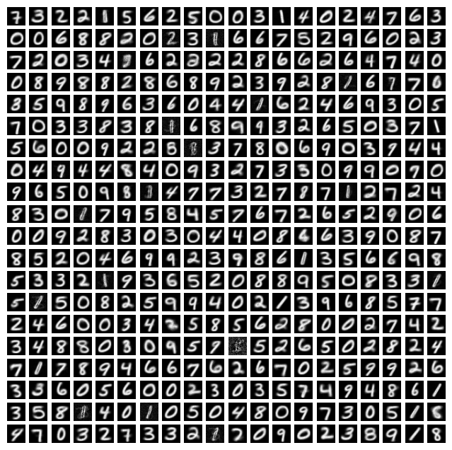
As you can see, most of these weights look like clearly discernable numbers. Each neuron is responsive to a particular digit (and a particularly way of drawing that digit). Each of these neurons is labeled according to the digit it responds to but we’ll pre-label them all.
We are also going to use pre-set firing thresholds for our excitatory neurons’ ALIFs. When we’re actually running our network, we will “freeze” both the STDP weights and the excitatory ALIFs’ firing thresholds.
Show code cell source
import zipfile
import json
import itertools
import random
from myst_nb import glue

random.seed(0)

def dataGenerator(path):
    with zipfile.ZipFile(path) as train_zip:
        with train_zip.open('index.json') as index_file:
            idx_info = json.loads(index_file.read())
            files = idx_info['files']
            N = idx_info['N']
            i = 0

            for fname in files:
                with train_zip.open(fname) as f:
                    data = json.loads(f.read())
                    images = data['images']
                    labels = data['labels']
                    for img, label in zip(images, labels):
                        yield (img, label)
                        i += 1
                        if i >= N: break

testDataGenerator = dataGenerator('../_static/datasets/test-chunked.zip')
Show code cell source
with open('../_static/datasets/theta.json') as theta_file:
    theta = json.loads(theta_file.read())
with open('../_static/datasets/neuron_labels.json') as labels_file:
    labels = json.loads(labels_file.read())

NUM_EXCITATORY = 400
TIME_TO_SHOW_IMAGES = 0.55 # seconds
TIME_TO_SHOW_BLANK  = 0.15 # seconds

# print(xeae)
t_step = 0.001  # Time step for the simulation
synapses = SynapseCollection(n=DIGIT_SIZE, tau_s=0.1, t_step=t_step)  # Synapse collection for input connections

# STDP (Spike-Timing-Dependent Plasticity) weight matrix between input and excitatory neurons
# stdp = STDPWeights(numPre=DIGIT_SIZE, numPost=NUM_EXCITATORY, g_min=-0.1, g_max=1.1)

# Inhibitory neurons and their corresponding post-synaptic potential (PSP) collection
inhibitory_neurons = LIF(n=NUM_EXCITATORY, t_step=t_step)
inhibitory_psp = SynapseCollection(n=NUM_EXCITATORY, t_step=t_step, tau_s=0.5)
inhibitory_outp = np.zeros(NUM_EXCITATORY)  # Initialize inhibitory output array

# Excitatory neurons and their corresponding PSP collection
excitatory_neurons = ALIF(n=NUM_EXCITATORY, t_step=t_step, tau_inh=1.1)
excitatory_neurons.inh = np.array(theta)
excitatory_psp = SynapseCollection(n=NUM_EXCITATORY, t_step=t_step, tau_s=0.2)

# Function to perform a simulation step
def step(inp, max_input_rate):
    global inhibitory_outp
    input_spikes = poisson_fire(np.array(inp), dt=t_step, min_rate=0.01, max_rate=max_input_rate)  # Generate input spikes
    input_psp = synapses.step(input_spikes)  # Step the input synapses to get PSP

    # stdp.step(t_step)  # Step the STDP mechanism
    # stdp.updateWeights(input_spikes, excitatory_neurons.output)  # Update weights based on input and output spikes

    # uses xeae as weights rather than stdp (assuming fixed weights)

    excitatory_inp = input_psp @ xeae + np.clip(inhibitory_outp * -1 / NUM_EXCITATORY, a_max=0, a_min=None)  # Calculate excitatory input combining synapse output and inhibitory output
    excitatory_spikes = excitatory_neurons.step(excitatory_inp)  # Step excitatory neurons to get their spikes

    excitatory_outp = excitatory_psp.step(excitatory_spikes)  # Update the excitatory post-synaptic potential

    inhibitory_spikes = inhibitory_neurons.step(excitatory_outp)  # Step inhibitory neurons using excitatory output
    # print(input_psp@stdp.w, excitatory_inp, excitatory_spikes, excitatory_outp, inhibitory_spikes)
    raw_inhibitory_outp = inhibitory_psp.step(inhibitory_spikes)  # Update the inhibitory post-synaptic potential
    total_inhibitory_outp = np.sum(raw_inhibitory_outp)  # Calculate the total inhibitory output
    inhibitory_outp = total_inhibitory_outp * np.ones(NUM_EXCITATORY) - raw_inhibitory_outp  # Calculate the inhibitory output for each neuron

    return excitatory_spikes > 0
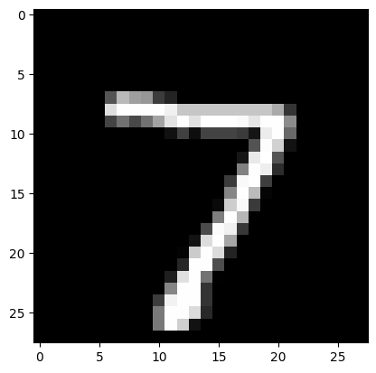
Then, we can run an example of our network classifying a new digit, highlighting the neuron(s) that fire most below (indicating that those are the neurons that “recognized” the digit).
Show code cell source
def run_simulation(num_images=1):
    for _ in range(num_images):
        current_image, label = next(testDataGenerator)  # Get the next image and label from the data generator

        total_fires = 0  # Initialize the total number of fires
        max_input_rate = 0.2  # Initial maximum input firing rate
        all_fires = np.zeros(NUM_EXCITATORY)  # Initialize the array to store all the fires
        max_fires = 0
        has_dominant_neuron = False

        while has_dominant_neuron == False and max_fires < 10:
            for _ in np.arange(0, TIME_TO_SHOW_IMAGES, t_step):  # Display the image for a set duration
                fires = step(np.array(current_image), max_input_rate=max_input_rate)  # Perform a simulation step
                all_fires += fires  # Accumulate the number of fires
                num_fires = np.sum(fires > 0)  # Calculate the number of fires
                total_fires += num_fires  # Accumulate the number of fires

                max_input_rate *= 1.1  # Increase the input firing rate
                max_fires = np.max(all_fires)
                has_dominant_neuron = np.sum(all_fires == max_fires) <= 1  # Check if there is a dominant neuron
                if has_dominant_neuron and max_fires >= 10: break


        for _ in np.arange(0, TIME_TO_SHOW_BLANK, t_step):  # Show a blank input for a set duration
            step(np.zeros(len(current_image)), max_input_rate=max_input_rate)  # Perform a simulation step with blank input

        dominant_idx = np.argmax(all_fires)
        predicted_label = labels[dominant_idx]
        print(f"Predicted Label: {predicted_label}, True Label: {label}")

        plt.figure()
        plt.imshow(np.array(current_image).reshape(DIGIT_WIDTH, DIGIT_HEIGHT), cmap="gray")
        plt.show()

        fig, axs = plt.subplots(NUM_NEURON_ROWS, NUM_NEURON_COLS, figsize=(8, 8))
        for i in range(NUM_NEURONS):
            ax = axs[i // NUM_NEURON_COLS, i % NUM_NEURON_COLS]
            ax.imshow(xeae[:, i].reshape(DIGIT_WIDTH, DIGIT_HEIGHT), cmap="gray" if all_fires[i] < max_fires else "hot")
            ax.axis("off")


run_simulation()

def plotWeights():
    NUM_DISPLAY_ROWS = 4
    NUM_DISPLAY_COLS = 4

    plt.figure()

    for i in range(NUM_EXCITATORY):
        plt.subplot(NUM_DISPLAY_ROWS, NUM_DISPLAY_COLS, i+1)
        plt.imshow(stdp.w[:, i].reshape(DIGIT_WIDTH, DIGIT_HEIGHT), cmap='gray')
        plt.axis('off')
    plt.show()
Predicted Label: 7, True Label: 7
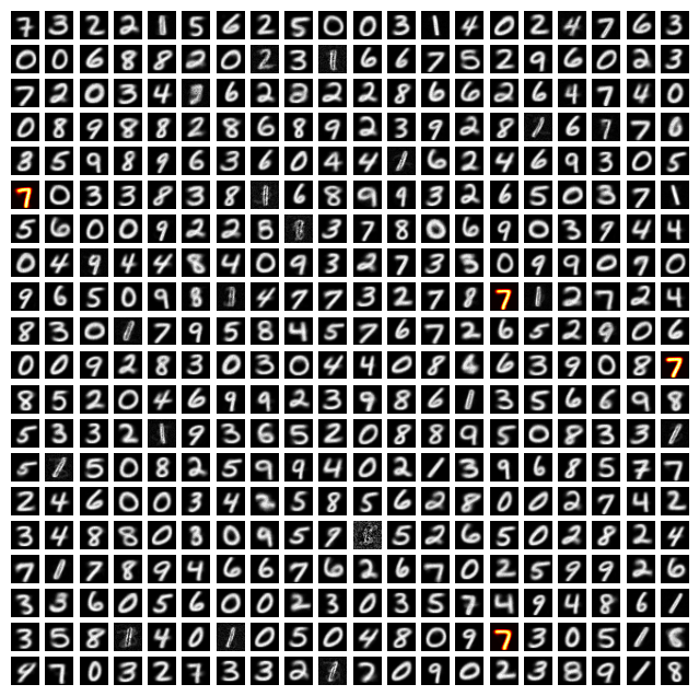
Our simulation worked well this time; the neurons that fired most were the ones that corresponded to the digit in the image (though the network is often inaccurate).
Summary#
We created a network that can recognize digits from the MNIST dataset
Our network uses primitives that we learned in prior notebooks: LIFs, ALIFs, STDP, and PSPs
The STDP weights, which we learn over time, encode the digits being recognized
Our network is a scaled down version of the one implemented by Diehl and Cook [DC15]
Note: This notebook (mostly) follows the paper: Diehl, Peter U., and Matthew Cook. “Unsupervised learning of digit recognition using spike-timing-dependent plasticity.” [DC15]